This article is the final part of my 3-part blog series about a project I made recently while learning Computer Vision which is about developing a complete Football Analytics Model using Yolov8 + BotSORT tracking.

Read the previous blogs here:

• https://medium.com/@nikhilc2209/an-image-annotation-guide-using-roboflow-for-object-detection-a4e30581b5cf
• https://medium.com/@nikhilc2209/player-and-ball-detection-using-yolov8-botsort-tracking-on-a-custom-dataset-19f84cfdacbf

Objective: This blog is about using the annotated frames from our Yolov8 model and further processing them to split the detected players into their respective teams based on their jersey colors using HSV Filtering.

A Brief look at the HSV Color space

The HSV Color space is an alternative to the popular and frequently used RGB Color space and is widely used in Image Processing and Computer Vision tasks. This is because it offers a lot more control in terms of lighting and brightness which is helpful in separating chromatic information from its intensity.

The HSV model stands for Hue Saturation and Value. Let's break down these 3 components:

• Hue: This component is responsible for discriminating between different colors. It is measured on a 360 degree scale which starts from red at 0 degree, green at 120 degrees, blue at 240 degrees and loops back again to red at 360 degrees.
• Saturation: Saturation refers to the intensity or purity of the color. A color with high saturation is vivid and rich, while a color with low saturation appears more muted or grayscale. This value is represented as a percentage from 0% to 100%.
• Brightness: The Value component represents the brightness or intensity of the color. This is also represented as a percentage value where 0% corresponds to black, while the maximum value 100% corresponds to the brightest possible color.

A condensed view of the HSV Color Space

What is HSV Filtering

HSV Filtering is the process of isolating and extracting specific colors from an image based on a pre-defined threshold of HSV values also known as masks. Let's work on a simple image to understand how this works:

Input Image

Let's use the above image and try to isolate and extract the flower from this image using OpenCV.

• First off we need to convert the given image from BGR to HSV color format, this is because OpenCV loads any image in the BGR format by default (yes, BGR not RGB format!). Read this article from OpenCV's CEO Satya Mallick about why OpenCV uses the BGR format by default: https://learnopencv.com/why-does-opencv-use-bgr-color-format/
• Next we need to define masks using the cv2.inRange() function which takes the hsv image as input and a pair of tuples with lower and upper threshold of hsv values for the target color. In our case, the target color is red so we'll define the masks accordingly.
• Another thing to keep in mind is that OpenCV uses a different range for HSV values, for Hue it is between (0-180), for saturation it is between (0-255) and for value it is again between (0-255).

Condensed view of the HSV Color map in OpenCV

• After defining threshold masks using the above image as reference, we can now use the bitwise_and operator from OpenCV to combine the binary mask with the input image to get the target color as the output.

1) Input Image 2) Thresholding Binary mask 3) Output Image after Bitwise_and operation

Using a hsv trackbar

Now we know how to create masks for isolating colors from our target image using the hsv color map, but creating masks for specific non-standard colors can be a bit tricky and can lead to dubious results. Therefore, we can use a hsv trackbar with sliders to change the hsv values of masks in real time to get the best possible output as shown below.

HSV trackbar in action

Ref.: https://stackoverflow.com/questions/44480131/python-opencv-hsv-range-finder-creating-trackbars

Storing all the jersey crops and color codes for each team

For the purpose of our project we'll only be working on teams from the Premier League, we can simply take a crop of jerseys of all the 20 teams and use our trackbar to log these values in a csv file. This way we can store hsv codes for all teams which includes home, away and third kit along with their respective goalkeeper kits.

The main idea behind using this approach to classify detected players into their respective teams is that football matches have teams with easily distinguishable jerseys to avoid clashes due to similar colors. We are simply leveraging this fact to our advantage as this applies to football matches all over the world.

Getting bounding box and label data from Yolov8 model

Now that we have built our color filtering module we'll go back to our tracking module and feed the results from the latter to the former to get the desired output. What we really need is bounding box co-ordinates for each detected player and their confidence score, we can use the bounding box co-ordinates and send crops of players to our hsv filtering module which will run it through all four masks (home & away team jersey, home & away goalkeeper jersey) and compute the output label.

To compute the output label we take masks for both the teams and their goalkeepers, then we can then simply count the number of non-black pixels for each output image resulting from each mask and choose the one with the maximum count.

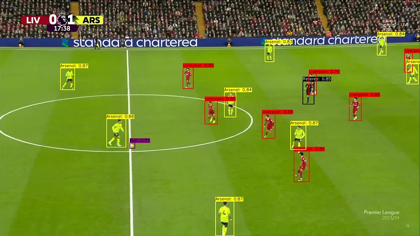
We can then draw bounding boxes using OpenCV with custom labels that we just computed which represent team names and their confidence scores. Looking at Ultralytics docs, to get the bounding box co-ordinates for each detected object we can use the results Class from each frame and use methods such as boxes.cls(), boxes.xyxy(), boxes.conf() to get the object label, its co-ordinates in xyxy format and its confidence score respectively.

Ref.: https://docs.ultralytics.com/reference/engine/results/

Saving results using OpenCV Videowriter

Now that we have plot our bounding boxes along with their custom labels for each frame we can simply compile these frames to produce the final output in video format. To do this we simply need to use the VideoWriter Class from OpenCV which takes in the following arguments:

result = cv2.VideoWriter('filename.avi', cv2.VideoWriter_fourcc(*'MJPG'), 10, size) 

# cv2.VideoWriter(filename, Codec Compression method, fps, frame_size(w,h))

Final Results

Source Code:

https://github.com/NikhilC2209/Football_Analytics_CV